Today I wanted to try my hand at a kaggle competition that seemed like another great place to practice using image neural networks. The competition asks us to identify humpback whales from their flukes (tail fins). Before getting into the model training, however, it's always important to look at your data. So let's do some basic exploratory data analysis (EDA) to better inform ourselves on just what our model will be looking at and attempting to train on.

Basic data exploration:

distribution of images per whale
viewing some images (same whale, different whale, 'new_whale')
distribution of image resolution between train & test
duplicate image analysis by perceptual hash

# used ideas from:
# https://www.kaggle.com/mmrosenb/whales-an-exploration 
# https://www.kaggle.com/stehai/duplicate-images
%reload_ext autoreload
%autoreload 2
%matplotlib inline

import numpy as np # linear algebra
import pandas as pd # data processing, CSV file I/O (e.g. pd.read_csv)
import cv2
import os
import seaborn as sns
import matplotlib.pyplot as plt
plt.rcParams['figure.figsize'] = [14, 9]

import collections
from PIL import Image

DIR = "../input"

train = pd.read_csv(os.path.join(DIR, "train.csv"))
test = pd.read_csv(os.path.join(DIR, "sample_submission.csv"))

train.shape, test.shape

((25361, 2), (7960, 2))

train.head()

	Image	Id
0	0000e88ab.jpg	w_f48451c
1	0001f9222.jpg	w_c3d896a
2	00029d126.jpg	w_20df2c5
3	00050a15a.jpg	new_whale
4	0005c1ef8.jpg	new_whale

Distribution of images per whale is highly skewed.

2000+ whales have just one (!!!) image
Single whale with most images have 73 of them
Images dsitribution:
almost 30% comes from whales with 4 or less images
almost 40% comes from 'new_whale' group (!!!)
the rest 30% comes from whales with 5-73 images

Let's look at how I figured out the above points. First let's look at the most populous whales in the dataset:

train['Id'].value_counts()[:4]

new_whale    9664
w_23a388d      73
w_9b5109b      65
w_9c506f6      62
Name: Id, dtype: int64

So this new_whale distinction appears to take up quite a bit of the dataset! Let's now see how many image per whale we can expect.

counted = train.groupby("Id").count().rename(columns={"Image":"image_count"})
counted.loc[counted["image_count"] > 80,'image_count'] = 80
plt.figure()
sns.countplot(data=counted, x="image_count")
plt.show()

png

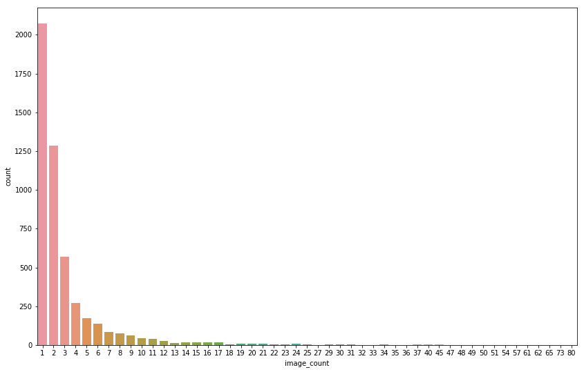
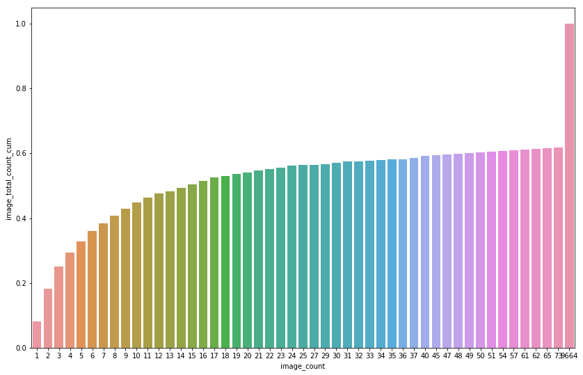
So it appears that a lot of the whales only have a few example images in the training set. Lets look at the cumulative totals to get an idea of the distribution.

image_count_for_whale = train.groupby("Id", as_index=False).count().rename(columns={"Image":"image_count"})
whale_count_for_image_count = image_count_for_whale.groupby("image_count", as_index=False).count().rename(columns={"Id":"whale_count"})
whale_count_for_image_count['image_total_count'] = whale_count_for_image_count['image_count'] * whale_count_for_image_count['whale_count']
whale_count_for_image_count['image_total_count_cum'] = whale_count_for_image_count["image_total_count"].cumsum() / len(train)
sns.barplot(x='image_count',y='image_total_count_cum',data=whale_count_for_image_count)

<matplotlib.axes._subplots.AxesSubplot at 0x7f1f03317128>

png

whale_count_for_image_count[:10]

	image_count	whale_count	image_total_count	image_total_count_cum
0	1	2073	2073	0.081740
1	2	1285	2570	0.183076
2	3	568	1704	0.250266
3	4	273	1092	0.293324
4	5	172	860	0.327235
5	6	136	816	0.359410
6	7	86	602	0.383147
7	8	76	608	0.407121
8	9	62	558	0.429123
9	10	46	460	0.447262

whale_count_for_image_count[-3:]

	image_count	whale_count	image_total_count	image_total_count_cum
46	65	1	65	0.616064
47	73	1	73	0.618942
48	9664	1	9664	1.000000

A few thoughts: 1. 'Typical' CNNs (e.g. resnet) are going to have difficulty learning from only 1-4 examples of each whale. This implies that we might want to try an alternative architecture for this task. One-shot learning seems to be related to this, I'll look into this further. 2. The new_whale category takes up over 40% of our training data. Will be interesting to see whether our model will have anyting to gain from these unknown whales or whether it would benefit us to just cut them from the dataset.

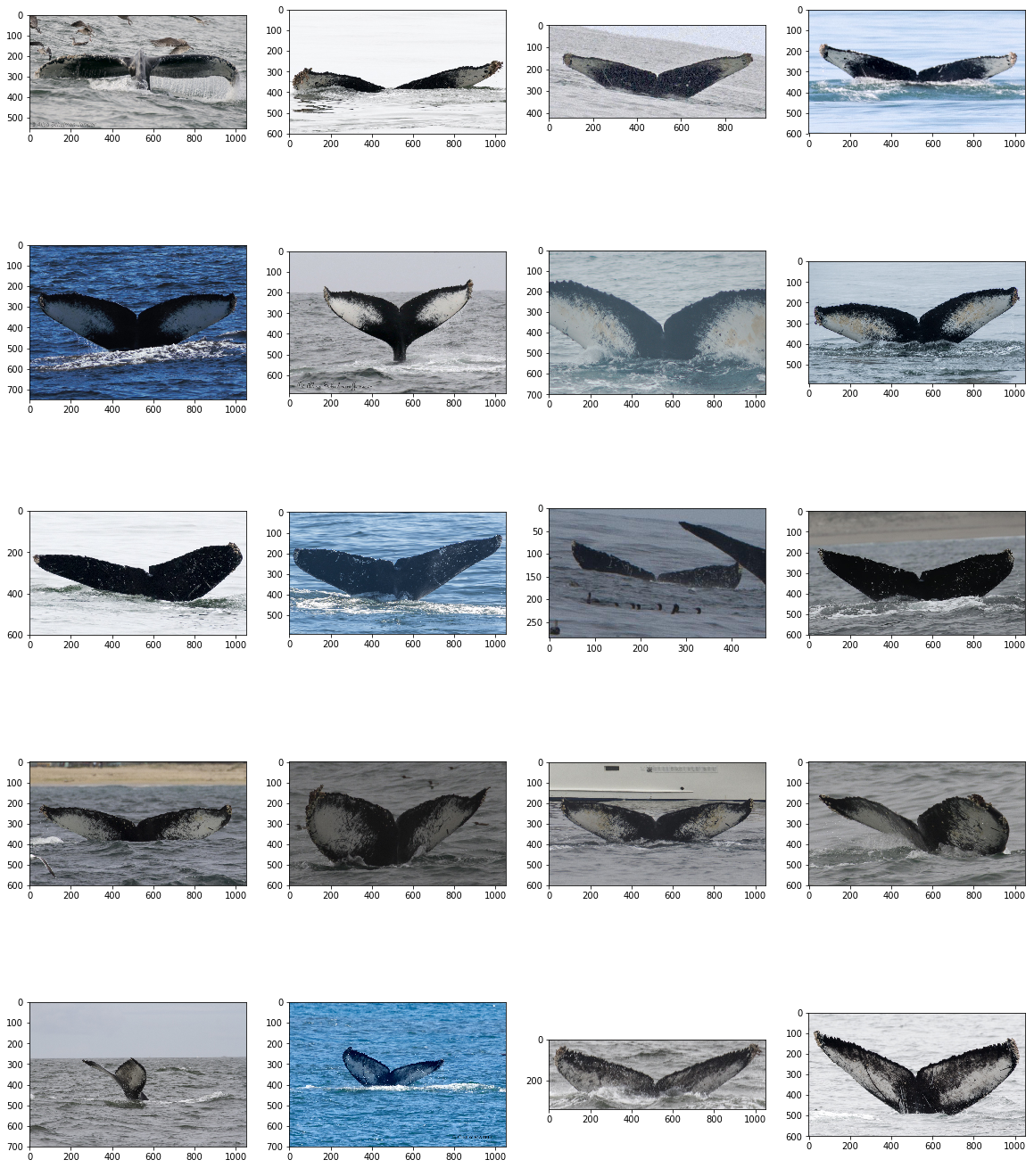
Let's see some images

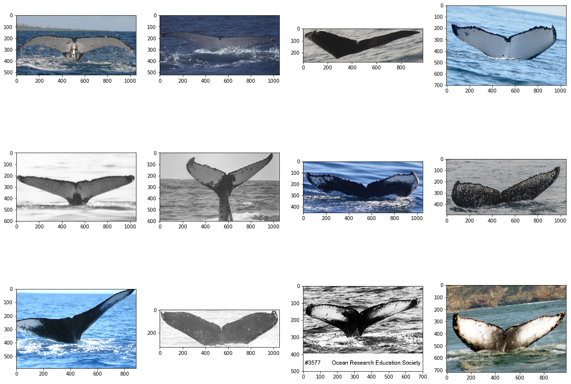
There are a wide range of images in the dataset. Large variety in color, colormaps (RGB vs black/white), image size and orientation of the image. Would greatly benefit from some standardization.
Looking at different images of one specific whale makes it seem like identification would be possible as they appear quite unique

Some images of 'new_whale'

fig = plt.figure(figsize = (20, 15))
for idx, img_name in enumerate(train[train['Id'] == 'new_whale']['Image'][:12]):
    y = fig.add_subplot(3, 4, idx+1)
    img = cv2.imread(os.path.join(DIR,"train",img_name))
    img = cv2.cvtColor(img, cv2.COLOR_BGR2RGB)
    y.imshow(img)

plt.show()

png

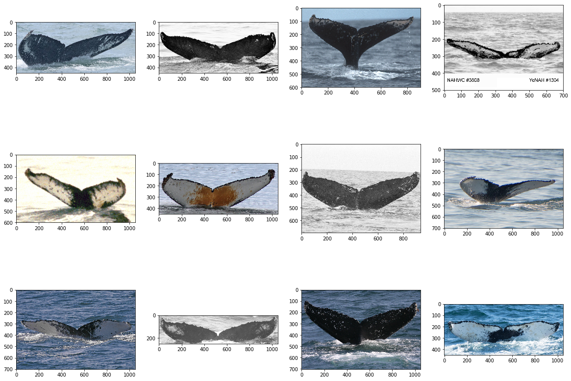
Now some pictures of whales that have just 1 image: quite a large variance in colors

single_whales = train['Id'].value_counts().index[-12:]
fig = plt.figure(figsize = (20, 15))

for widx, whale in enumerate(single_whales):
    for idx, img_name in enumerate(train[train['Id'] == whale]['Image'][:1]):
        axes = widx + idx + 1
        y = fig.add_subplot(3, 4, axes)
        img = cv2.imread(os.path.join(DIR,"train",img_name))
        img = cv2.cvtColor(img, cv2.COLOR_BGR2RGB)
        y.imshow(img)

plt.show()

png

Below: each row shows pictures of one whale. I think it's quite easy to at least see similiar appearence there

topN=5
top_whales = train['Id'].value_counts().index[1:1+topN]
fig = plt.figure(figsize = (20, 5*topN))

for widx, whale in enumerate(top_whales):
    for idx, img_name in enumerate(train[train['Id'] == whale]['Image'][:4]):
        axes = widx*4 + idx+1
        y = fig.add_subplot(topN, 4, axes)
        img = cv2.imread(os.path.join(DIR,"train",img_name))
        img = cv2.cvtColor(img, cv2.COLOR_BGR2RGB)
        y.imshow(img)

plt.show()

png

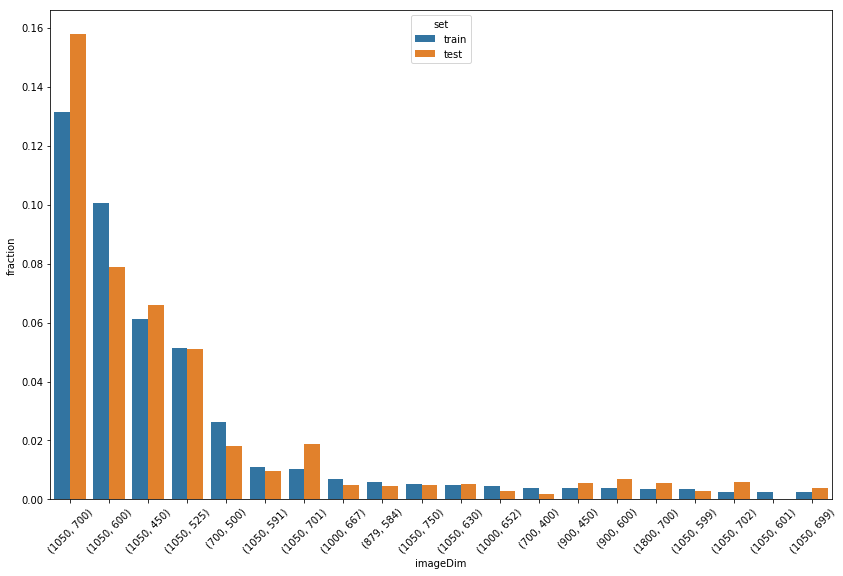
Resolutions

over 7000 unique resolutions but 39 most popular cover ~45% images (both in train and in test)

imageSizes_train = collections.Counter([Image.open(f'{DIR}/train/{filename}').size
                        for filename in os.listdir(f"{DIR}/train")])
imageSizes_test = collections.Counter([Image.open(f'{DIR}/test/{filename}').size
                        for filename in os.listdir(f"{DIR}/test")])

def isdf(imageSizes):
    imageSizeFrame = pd.DataFrame(list(imageSizes.most_common()),columns = ["imageDim","count"])
    imageSizeFrame['fraction'] = imageSizeFrame['count'] / sum(imageSizes.values())
    imageSizeFrame['count_cum'] = imageSizeFrame['count'].cumsum()
    imageSizeFrame['count_cum_fraction'] = imageSizeFrame['count_cum'] / sum(imageSizes.values())
    return imageSizeFrame

train_isdf = isdf(imageSizes_train)
train_isdf['set'] = 'train'
test_isdf = isdf(imageSizes_test)
test_isdf['set'] = 'test'

isizes = train_isdf.merge(test_isdf, how="outer", on="imageDim")
isizes['total_count'] = isizes['count_x'] + isizes['count_y']
dims_order = isizes.sort_values('total_count', ascending=False)[['imageDim']]
len(dims_order)

isizes = pd.concat([train_isdf, test_isdf])

isizes.shape

(8150, 6)

isizes.head()

	imageDim	count	fraction	count_cum	count_cum_fraction	set
0	(1050, 700)	3330	0.131304	3330	0.131304	train
1	(1050, 600)	2549	0.100509	5879	0.231813	train
2	(1050, 450)	1556	0.061354	7435	0.293167	train
3	(1050, 525)	1303	0.051378	8738	0.344545	train
4	(700, 500)	667	0.026300	9405	0.370845	train

popularSizes = isizes[isizes['fraction'] > 0.002]
popularSizes.shape

(39, 6)

popularSizes.groupby('set').max()['count_cum_fraction']

set
test     0.456030
train    0.445803
Name: count_cum_fraction, dtype: float64

sns.barplot(x='imageDim',y='fraction',data = popularSizes, hue="set")
_ = plt.xticks(rotation=45)

png

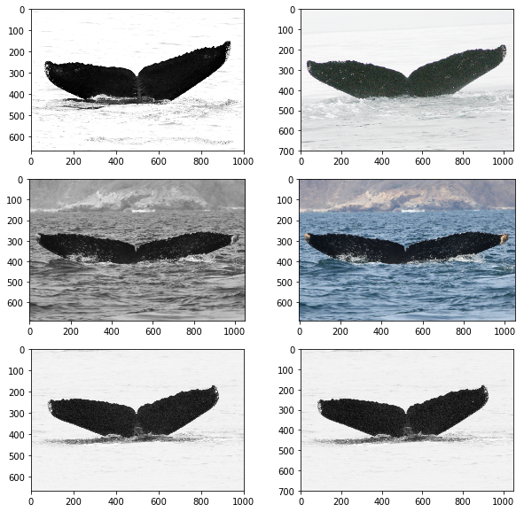
Duplicates

Found duplicates using imagehash. Great introduction here
1 duplicate in train set
3 duplicates between train and test
totally different than in playground dataset:
playground duplicates
solution that used duplicate information

import imagehash

def getImageMetaData(file_path):
    with Image.open(file_path) as img:
        img_hash = imagehash.phash(img)
        return img.size, img.mode, img_hash

def get_img_duplicates_info(df, dataset):

    m = df.Image.apply(lambda x: getImageMetaData(os.path.join(DIR, dataset, x)))
    df["Hash"] = [str(i[2]) for i in m]
    df["Shape"] = [i[0] for i in m]
    df["Mode"] = [str(i[1]) for i in m]
    df["Length"] = df["Shape"].apply(lambda x: x[0]*x[1])
    df["Ratio"] = df["Shape"].apply(lambda x: x[0]/x[1])
    df["New_Whale"] = df.Id == "new_whale"


    img_counts = df.Id.value_counts().to_dict()
    df["Id_Count"] = df.Id.apply(lambda x: img_counts[x])
    return df

train_dups = get_img_duplicates_info(train, "train")

train_dups.head()

	Image	Id	Hash	Shape	Mode	Length	Ratio	New_Whale	Id_Count
0	0000e88ab.jpg	w_f48451c	d26698c3271c757c	(1050, 700)	RGB	735000	1.500000	False	14
1	0001f9222.jpg	w_c3d896a	ba8cc231ad489b77	(758, 325)	RGB	246350	2.332308	False	4
2	00029d126.jpg	w_20df2c5	bbcad234a52d0f0b	(1050, 497)	RGB	521850	2.112676	False	4
3	00050a15a.jpg	new_whale	c09ae7dc09f33a29	(1050, 525)	RGB	551250	2.000000	True	9664
4	0005c1ef8.jpg	new_whale	d02f65ba9f74a08a	(1050, 525)	RGB	551250	2.000000	True	9664

t = train_dups.Hash.value_counts()
t = t.loc[t>1]

"Duplicate hashes: {}".format(len(t))

'Duplicate hashes: 1'

94216bb289ccd63f    2
Name: Hash, dtype: int64

t.index[0]

'94216bb289ccd63f'

train_dups[train_dups['Hash'] == t.index[0]].head()

	Image	Id	Hash	Shape	Mode	Length	Ratio	New_Whale	Id_Count
9542	60a3f2422.jpg	w_7a8ce16	94216bb289ccd63f	(1050, 525)	RGB	551250	2.0	False	6
12618	7f7a63b8a.jpg	w_7a8ce16	94216bb289ccd63f	(1050, 525)	RGB	551250	2.0	False	6

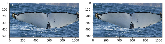
The only duplicate found in train dataset comes from the same whale.

fig = plt.figure(figsize = (20, 10))
for idx, img_name in enumerate(train_dups[train_dups['Hash'] == t.index[0]]['Image'][:2]):
    y = fig.add_subplot(3, 4, idx+1)
    img = cv2.imread(os.path.join(DIR,"train",img_name))
    img = cv2.cvtColor(img, cv2.COLOR_BGR2RGB)
    y.imshow(img)

plt.show()

png

test_dups = get_img_duplicates_info(test, "test")

test_d = test_dups.Hash.value_counts()
test_d = test_d.loc[test_d>1]
"Duplicate hashes in test: {}".format(len(test_d))

'Duplicate hashes in test: 0'

common_hashes = test_dups.merge(train_dups, how="inner", on="Hash", suffixes=("_test","_train"))
common_hashes.head()

	Image_test	Id_test	Hash	Shape_test	Mode_test	Length_test	Ratio_test	New_Whale_test	Id_Count_test	Image_train	Id_train	Shape_train	Mode_train	Length_train	Ratio_train	New_Whale_train	Id_Count_train
0	d37179fd1.jpg	new_whale w_23a388d w_9b5109b w_9c506f6 w_0369a5c	eecad0b52d4ac2f0	(1050, 700)	RGB	735000	1.500000	False	7960	01f66ca26.jpg	new_whale	(1000, 667)	RGB	667000	1.499250	True	9664
1	f50529c53.jpg	new_whale w_23a388d w_9b5109b w_9c506f6 w_0369a5c	afdac0b52a5a82b5	(1050, 690)	RGB	724500	1.521739	False	7960	579886448.jpg	new_whale	(1050, 690)	RGB	724500	1.521739	True	9664
2	fb3879dc7.jpg	new_whale w_23a388d w_9b5109b w_9c506f6 w_0369a5c	ad4ac2b43d0fcaf0	(1050, 700)	RGB	735000	1.500000	False	7960	b95d73a55.jpg	w_691f2f6	(1000, 667)	RGB	667000	1.499250	False	8

"Duplicate hashes between train and test: {}".format(len(common_hashes))

'Duplicate hashes between train and test: 3'

below each row shows images with the same pHash, left column from train, right from test

fig = plt.figure(figsize = (10, 10))

for idx, images in enumerate(common_hashes[['Image_train','Image_test']].values):
    y = fig.add_subplot(len(common_hashes),2, idx*2+1)
    img = cv2.imread(os.path.join(DIR,"train",images[0]))
    img = cv2.cvtColor(img, cv2.COLOR_BGR2RGB)
    y.imshow(img)

    y = fig.add_subplot(len(common_hashes),2, idx*2+2)
    img = cv2.imread(os.path.join(DIR,"test",images[1]))
    img = cv2.cvtColor(img, cv2.COLOR_BGR2RGB)
    y.imshow(img)


plt.show()

png

# train duplicates - to remove:
train_to_remove = train_dups[train_dups['Hash'] == t.index[0]].drop_duplicates('Hash')[['Image']]
train_to_remove.to_csv("train_remove.csv",index=False)
train_to_remove.head()

	Image
9542	60a3f2422.jpg

# easy answers in test:
easy_peasy = common_hashes[['Image_test','Id_train']]
easy_peasy.to_csv("test_easy.csv", index=False)
easy_peasy.head()

	Image_test	Id_train
0	d37179fd1.jpg	new_whale
1	f50529c53.jpg	new_whale
2	fb3879dc7.jpg	w_691f2f6

Conclusion

Just by poking around the dataset I've gained quite a bit of insight on how we're going to tackle this problem. My next step is going to be cleaning and standardizing the dataset, to make it easier to train on. Then, I'll need to find an architecture that is the best suited for learning off of very few examples. I'm not sure if such an architecture exists but I'll report back with what I find!

Getting to know humpback whales with EDA

November 11, 2018